Google Sheets is a powerful and free tool for managing complex spreadsheets. This tutorial dives into ten useful formulas you must know to help you simplify the way you work in Google Sheets.

GOOGLEFINANCE
This function returns market information from Google Finance related to a specific company.
=GOOGLEFINANCE(symbol, attribute)
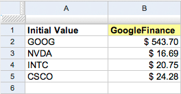
For example, if you want to know the Google stock price, copy and paste the following formula into the cell B2:
=GOOGLEFINANCE(A2,"price")
You can use the same formula for the other companies in this example (NVidia, Intel, Cisco,…). Other attributes are volume, earning per share, opening price, and so on (take a look at the official documentation for a full list).
You can also use it to look up current crypto prices, such as Bitcoin and Ethereum.
=GOOGLEFINANCE("BTCUSD")
However, GOOGLEFINANCE doesn’t support all cryptocurrencies yet. For others, I recommend using cryptoprices.cc. Here is an example looking up the current price of Solana.
=IMPORTDATA("https://cryptoprices.cc/SOL/")
Vertical Look Up
This formula searches for value in the left-most column of array and returns the value in the same row based on the index.
=vlookup(search_criterion, array, index, sort_order)

For example, if you want to find the population of the value contained in the cell C2, from all values contained in the range A2:B4, copy and paste the following formula into the cell D2:
=vlookup(C2;A2:B4;2;false)
Filter
This formula returns a filtered version of the given source array.
=filter(range; condition1, condition2,...)
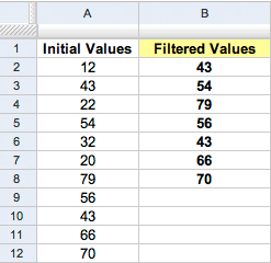
In this example I filtered all values contained in the column A (rangeA2:A12) greater than 37.
Copy and paste the following formula into the cell B2:
=filter(A2:A12;A2:A12>37)
You can also use multiple conditions to filter a source array:
=filter(A2:A12;A2:A12>37; A2:A12<60)
In this case, the formula returns all values contained in the range A2:A12 greater than 37 AND less than 60.
Concatenate
This function concatenates several text strings, contained in different cells, into one string.
=concatenate(text1, text2, text3,…)
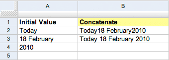
If you want to concatenate all values contained in the cells A2, A3, A4 into one string, copy and paste this formula into the cell B2:
=concatenate(A2,A3,A4)
If you want to separate every single value with a space (cell B3), use this formula:
=concatenate(A2," ", A3," ", A4)
Find
This formula looks for a string of text within another string and returns an integer.
=find(find_text, text, position)

For example, if you want to find the “space” within the string contained in the cell C2 (which contains this text: Jack Bauer), copy and paste the following formula into the cell B2:
=find(" ", A2, 1)
This formula returns “5” that means the “space” is found within the source string after 4 characters.
Left and Right
Left extracts a substring from a string, starting from the left-most character.
=left(text, number)
Right extracts a substring from a string, starting from the right-most character.
=right(text, number)
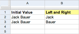
If you want to extract the name “Jack” from the cell A2, copy and paste the following formula into the cell B2:
=left(A2;4)
If you want to extract the surname “Bauer” from the cell A3, copy and paste the following formula into the cell B3:
=right(A3;5)
You can also use the following formula to extract dynamically the name from an array of multiple values (Jack Bauer, Gregory House, Christian Troy, …):
=left(A2; find(" ", A2, 1)-1)
Split
This formula splits text based on the given delimiter, putting each section into a separate column in the row.
=split(string, delimiter)

For example, if you want to split the values contained in the column A, using the delimiter ” ” (space), copy the following formula into the column B (the column C will be populated automatically):
=split(A2," ")
Substitute
This formula substitutes new text for old text in a string.
=substitute(text, search_text, new text, occurrence)
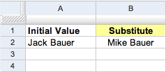
If you want to substitute “Jack” with “Mike” from the text contained in the cell A2, copy and paste this formula into the cell B2:
=substitute(text, search_text, new text, occurrence)
Occurrence (optional, in this case “1”) indicates how many occurrences of the search text are to be replaced.
Unique
This formula returns only the unique values in the source array, discarding duplicates.
=unique(array)
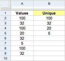
If you want to obtain an array of unique values from the values contained in the column A, copy and paste the following formula into the cell B2:
=unique(A2;A9)
As you can see, this formula returns only unique values in the column A, discarding all duplicates.
GOOGLELOOKUP
Note: This is no longer available. If you have a good alternative, feel free to drop it below in the comments, and I’ll get this section updated.
This formula attempts to find the values for straightforward facts about specific things.
=GOOGLELOOKUP(entity, attribute)
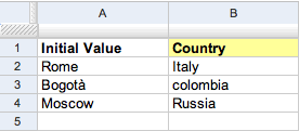
For example, if you want to find the countries of cities listed in the column A, copy and paste the following formula into the column B:
=GOOGLELOOKUP(A2;"country")
You can access some types of entities such as countries and territories (population, largest city), rivers (origin, length), actors and musicians (date of birth, nationality), planets, and so on. For a full list of popular entities, take a look at the official documentation.
GoogleLookup was discontinued in 2011… did you just pull this from other blogs without doing any of your own research?
Hey Cock,
This was originally published in February 2010. Nope, I always do my own research. If you have an alternative for GoogleLookup, feel free to leave a constructive comment, and I’ll get it updated.
Here’s your constructive comment: when someone informs you that something in the article wasn’t even true the moment you (re)publicized it, remove it from the article. Or at the very least add an update to it.
This was never republished and has been live since 2010 (across different domains), as I already mentioned above. It’s crazy how many people make assumptions these days. If you have an alternative for GoogleLookup, happy to update it. Feel free to drop in a comment. But you’re just wasting your time if you can’t leave a constructive comment with a solution. Everybody loves to complain, but yet they don’t actually provide any useful feedback.